Morning Desk Quant: mathematics, decisions, and learning
Protocol quant-desk-v1 · specified 20 November 2026 · implementation: engine/quant-desk.mjs, engine/quant/learning.mjs.
This document describes the implemented estimator and decision policy. The formulas are not claims of profitable performance. The dashboard supplies measured results when the data job succeeds; synthetic test fixtures never become production evidence.
1. Information, clocks, and what “yesterday” means
Let  denote information available at the close of trading session
 . A valid decision
 is measurable with respect to . If today's New York date is
 , this implementation uses only bars with date strictly less than , even if today's close has occurred. The latest retained SPY date is shown as
dataThrough.
The four horizons are  observed SPY trading sessions. Calendar month lengths and weekends are not silently treated as trading days. Features use trailing 1/5/21/126 observations; review windows select outcomes that finished in the last 1/5/21/126 SPY sessions. A six-month forecast is not scored until 126 sessions have completed. Pending outcomes are neither losses nor wins.
The system requests ten years of daily history to obtain multiple regimes and enough historical comparisons. The latest six months alone contain approximately one disjoint six-month outcome per asset. Correlated stocks do not turn that single episode into hundreds of independent experiments.
2. Return labels, prices, and executable timing
Let  be the split-adjusted close,
 the dividend-adjusted close, and
 the opening price. Define the adjustment factor
 when adjusted observations exist for the entire retained series. Otherwise use price returns and explicitly label the basis
price-only.
For a signal at close , the standardized historical exposure enters at the next session's open and exits at close  :

For a long exposure with per-side cost  (5 basis points), the additive cost approximation is

Costs stand for spread/slippage. The report repeats the calculation at twice and four times the assumed cost. This is a transparent assumption, not a measured execution-cost model. No commissions, taxes, market impact or financing are inferred. Missing actual opens cannot be replaced with closes for evaluation.
The same-date SPY comparison is  ; equal round-trip cost assumptions cancel in that difference. An absolute win is distinct from beating SPY. Cash earns zero in this comparison.
For a recorded sell/trim/avoid decision, the diagnostic is avoided return,  , relative to continuing to hold. It is NOT short-sale profit, a full-account return or a simulation of a partial trim. Both positive and negative diagnostics are shown. Pending limit or breakout orders are not claimed to have filled. Fixed-horizon diagnostics do not implement the desk's stop/target path; the existing swing backtest remains the place to evaluate those rules.
Recorded calls receive a conservative uniform timing rule: the first full SPY session strictly after the issue date. A pre-open recorded call therefore also waits one session. This avoids claiming an execution before a call's actual creation time.
3. Predeclared strategies and market features
For  define
 . The 20-session volatility is the sample standard deviation of daily log returns multiplied by
 :

The four fixed long-entry hypotheses are:
| Strategy | Required conditions |
|---|---|
| Persistent trend |  ,  , price above its 200-session moving average |
| Pullback | , price above 200-session average,  |
| Relative momentum |  ,  , price above 50-session average |
| Volatility-filtered trend | , price above 200-session average,  |
A false condition means no entry for that strategy. It is not a bearish trade. No model searches thresholds to maximize the displayed backtest. Sector ETFs and individual stocks provide separate observable inputs; these technical rules do not infer valuation from prices or replace the existing earnings/macro research.
TQQQ and SQQQ are researched using their own traded histories. Their multi-day returns are never fabricated as a fixed multiple of QQQ. Leveraged and inverse instruments stay outside the live allocation mandate and do not earn a live tilt.
4. Walk-forward probabilities and expected returns
At each historical signal time, the training set is

The strict inequality purges labels that end on or after the signal date. Predictions are produced before the next outcome is appended to the learner. Signal cohorts are spaced  SPY sessions apart; all stocks entering together stay in the same cohort.
Given  matured training observations and
 wins, the probability point estimate is

Under an IID Bernoulli model with a  prior, this is the posterior mean. Real returns are not IID: here it is a regularized point estimate. We do NOT interpret the narrow IID beta interval as reliable market uncertainty. Uncertainty is estimated by joint time-block resampling instead.
The predicted net return uses shrinkage toward zero:
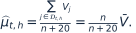
Both shrinkage constants are protocol parameters, not optimized after inspecting results. At  , the numerical priors are
 and
 , not evidence of a 50% trading advantage. Reported prequential performance excludes predictions with fewer than 30 training observations. The interface separately reports the number of independent entry-date cohorts.
A pooled rule probability refers to that rule's selected universe. It is not automatically the conditional probability for one ticker. Current symbol forecasts are labeled with their conditioning basis; small symbol samples remain uncertain.
5. Probability loss, return loss, and calibration
For predictions saved before outcomes, the Brier score and binary log loss are
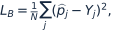

For numerical stability log-loss probabilities are clipped to  . The constant 0.5 probability baseline has Brier score 0.25. Its baseline is a useful reference, not a competitive market model. Five reliability bins compare average predicted probability with observed frequency.
Why use a proper score? If the true event probability is  , expected Brier loss satisfies

Its unique minimizer is  . A forecaster is rewarded for calibrated uncertainty, not for pretending certainty.
For return predictions, use

and compare with  , the zero-return predictor. A strategy can have high win frequency and negative expected return:
 . Therefore admission never depends on win rate alone.
6. Dependence, uncertainty, and multiple comparisons
Rolling 126-session outcomes share most of their daily returns. Counting them as independent would exaggerate confidence. Historical rule evaluations use disjoint horizon cohorts. For recorded calls, the engine greedily retains non-overlapping calendar intervals across the entire panel. The ledger retains every frozen call. Watch ideas, unfilled conditional entries and mandate exits are excluded from directional learning.
For uncertainty, keep every asset from an entry date together and sample circular blocks of three consecutive cohorts. Recompute the mean and regularized win estimate over 199 bootstrap samples; report their 2.5th and 97.5th percentiles. These intervals preserve some cross-asset and serial dependence, but remain approximate, particularly for sparse regimes. Fewer than five cohorts produces no interval. Thirty cohorts is the minimum for a learned policy adjustment, not a universal statistical guarantee.
For a benchmark-excess significance check, average excess within each date cohort, giving  . With
 cohorts and lag length
 :


The normal approximation to  supplies a one-sided p-value for positive excess. Fewer than 20 cohorts is untestable. This is a small-sample approximation, not proof of a causal relation.
Across the predeclared strategy/horizon comparisons, Holm's step-down rule orders p-values  and rejects sequentially while
 . Stop at the first failure. Untestable comparisons cannot pass.
Admission also requires 30 cohorts, a positive lower bootstrap bound on ordinary-instrument excess, and positive mean return at twice assumed costs. Passing these conditions does not establish a future guarantee or remove universe-selection bias.
The 95% expected shortfall diagnostic is the negative average of the worst 5% of observed net exposure returns. It is a horizon-specific empirical loss measure, not portfolio VaR. It can be negative if even the worst observed returns were positive. The dashboard does not annualize overlapping trades into an invented Sharpe ratio or CAGR.
7. The implemented “brain update”
The model's neural-network parameters are not retrained. Each successful daily quant report stores an immutable policy version and a compact learning summary. Future API analyst prompts receive that summary. Hand-in analysts can read /api/quant; their templates require this before the next report. An external task must actually read it—changing a template is not a claim that another service's saved task has been edited.
Among admitted monthly strategies, weights are normalized loss-based weights:
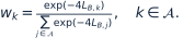
Non-admitted strategies have zero weight. For symbol  , the learned committee addition is

No admitted strategy means zero additional tilt. The maximum is 0.15. A positive research tilt never overrides account, sector, instrument or earnings restrictions. This bounded mechanism is a specified policy; the adaptive ensemble itself has not yet accumulated a prospective track record.
Each analyst desk starts with reliability multiplier 1. Only after at least 30 non-overlapping monthly long-call cohorts, with a negative upper bootstrap bound on net return, is its multiplier reduced to 0.75. The analyst component averages the attenuated votes over the original number of votes. A similarly poor prospective committee record reduces new-idea risk to 75% of the usual size. It never raises the original account risk ceiling. Historical rule replays and retrospective legacy calls cannot trigger these live reliability/risk reductions.
Policies use completed data before the decision's date and expire for decision use after four calendar days. A stale/missing report leaves baseline policy in place and is marked in the decision response. This is not an automatic sell mechanism.
8. Immutable decisions and counterfactual review
The first observed source/symbol/horizon call of a session is appended with its actual issue timestamp, action, horizon, model version and then-available empirical probability. Later same-day changes cannot overwrite it. All four horizons are stored independently. Probabilities are null while a source lacks sufficient prospective history; conviction is never recoded as a probability.
The daily counterfactual report asks whether taking long exposure or staying in cash did better over the specified horizon. A sell/avoid call is compared with continuing to hold. “The opposite action did better” describes a realized outcome; it does not prove that the opposite action was the right ex-ante decision. The same thesis can lose over one day and win over six months. The desk must evaluate it on its intended horizon, while showing all horizons for diagnosis.
Old entries from the mutable calls table are shown as retrospective diagnostics without forecast loss. Their missing issue-time provenance cannot be repaired honestly. They never train live desk weights. Actual account performance still requires broker fills, cash flows and a cash/position ledger; this feature does not invent them.
9. Limits and extension boundaries
The selected present-day universe contains survivorship and selection bias. Historical adjusted prices are current vendor reconstructions, not a point-in-time data archive. Price-only sources omit dividends. Data failures and omitted symbols are visible, rather than silently filled with simulated returns.
These are daily research and fixed-horizon models. No intraday edge, options pricing arbitrage, executable short strategy, optimal portfolio solver, HFT infrastructure or guaranteed alert latency is claimed. Existing options analytics, fundamental research, portfolio construction and stop/target backtests remain separate inputs. The 126-session horizon may correctly display insufficient independent outcomes for a long time.
Next extensions require separate protocols and validation: point-in-time fundamentals, delisted securities, measured execution costs, a locked holdout for the adaptive ensemble, regime-conditioned probability calibration, and a fill-based portfolio ledger. None is labeled implemented here.
References
- Gneiting and Raftery, Strictly Proper Scoring Rules, Prediction, and Estimation (2007): https://sites.stat.washington.edu/raftery/Research/PDF/Gneiting2007jasa.pdf
- Newey and West, A Simple, Positive Semi-Definite, Heteroskedasticity and Autocorrelation Consistent Covariance Matrix: https://www.nber.org/papers/t0055
- scikit-learn, chronological cross-validation and gaps: https://scikit-learn.org/stable/modules/generated/sklearn.model_selection.TimeSeriesSplit.html
The implementation combines these statistical ideas with explicitly chosen engineering rules. The sources do not endorse Morning Desk or imply that its strategies work.
The desk withholds all strategy tilts when any predeclared symbol is missing the most recent market session.